
ModelVision software, Research and Services
Acerca de
ModelVision Knowledge Base
Body Labels
Sometimes it is difficult to move body labels without grabbing/moving the body as well, despite the handles being displayed on the body.
When moving the Body Label hold the CTRL key down while clicking the left mouse button.
How can I compute the Magnetic Field of a project area?
To compute the Magnetic Field (i.e. Total Intensity, Inclination and Declination) you must know the Latitude and Longitude of the project area.
Access the Project Properties dialog from the File>Project Properties menu option and select the IGRF button on the right-hand side of the dialog. Choose a localised map from the drop-down list in the IGRF dialog that appears and click on the map in the area of the project.
Alternatively enter the Latitude/Longitude/Altitude of the project area and click OK. The Magnetic Field is then automatically calculated.
How can I determine the volume of a modelled body?
The volume of a created tabular or polygonal body in ModelVision is automatically calculated during the modelling process. The resultant value can be viewed in the Body Properties dialog.
To access the Body Properties dialog double-click the left mouse button on the target body in any view. Alternatively view the Body Table (accessed from the Model>Body Operations menu option) and double-click with the left mouse button on the row header cell of the target body.
How can I show my drillholes in a cross-section view?
To show either synthetic or imported drillholes in a cross-section view access the Cross-section Layer Table by clicking on the Layer Table toolbar button or right mouse button within the active cross-section window and choose the Configure Layers option from the pop-up menu. Then right click on the Cross-section Layers table to select Add>Drillhole. Move the drillholes that you wish to display to the Selected list on the right-hand side of the Drillhole Selection dialog. Click OK to return to the cross-section view to see the added drillholes.
How do I not display the Flight Lines or Base Lines in a 2D Map?
Turn off the display of survey database flight lines or base lines from the Map Layers Table. Access this by clicking on the Layer Table toolbar button or right mouse button within the active map and select the Configure Layers option from the pop-up menu. In the Map Layers Table deselect the tick boxes for Baselines and /or Flight Lines.
How can I set the background density or susceptibility?
The default background density and susceptibility values are set to 2.65 (mgal) and 0.0000 (cgs) respectively but can be changed by accessing the Model Parameters dialog from the Project Properties dialog, which is accessed from the File>Project Properties menu option. In the Project Properties dialog select the Model button on the left-hand side to display the Model Parameters dialog.
The Model Parameters dialog can also be accessed from the Model>Model Parameters menu option.
The default modelled density and susceptibility values are also defined in this dialog and are set to 2.77 (mgal) and 0.001 (cgs) respectively.
How can I set the default units for density and susceptibility?
The default density and susceptibility units are set to mgal and cgs by default. These units can be changed by accessing the Project Properties dialog from the File>Project Properties menu option and changing the units for Mag Units and Grav Units.
How can I produce a spreadsheet of my modelled bodies and their properties?
You can view a spreadsheet of the modelled bodies and their associated properties by selecting the File>Export>CSV Format menu option.
How can I load a DXF file into ModelVision?
Any external DXF or TKM (ModelVision format) file for a model can be imported into ModelVision by using the Model>Import menu option.
When importing a DXF file, the ModelVision Topology Checker dialog will appear, providing a preview of the model and checking the integrity of the model. If any unclosed edges, etc are detected these are reported and not imported.
How can I improve the speed of modelling in my session?
The speed at which ModelVision can model magnetic or gravity anomalies depends upon how many data points are being used in the session. Therefore, to increase the modelling efficiency of the software, it is advisable to isolate the area that is being modelled.
Use the Clip Project toolbar button to drag out a rectangular polygon of the area that you wish to clip to and click OK on the confirm dialog that appears. Note: once the data has been clipped you will not be able to display the full dataset again in the current session. Therefore, it is advisable to save the session for future use prior to clipping the project.
How to perform terrain corrections in ModelVision
When conducting gravity surveys, it is necessary to correct for the effect of terrain. Terrain correction is usually done by calculating the forward model of the terrain using a constant density. This effect is then removed from the gravity response as one of the corrections performed when processing raw gravity into a product used for interpretation. The usual approach is to convert the terrain into a body by faceting the terrain surface and giving it some thickness down to a flat base level below the lowest elevation value. The extents of this body need to be extended out from the margins of the survey to avoid edge effects.
There are three methods which ModelVision provides to compute terrain correction.
1. Terrain Correction Calculator
The Terrain Correction calculator is found in the Tools menu. One approach to faceting this body is to use a constant mesh width over the whole of the terrain. However, the response from distant terrain variations have less effect than close variations. When using constant facet dimensions over the whole terrain, calculation time is wasted calculating a fine response at distance when a coarse mesh could be used at distance with negligible impact. Using the fine mesh everywhere takes a considerable time to calculate, especially for large surveys. The terrain correction calculator in ModelVision significantly reduces the amount of calculation time needed by using larger mesh sizes at larger distances from the calculation point.
The algorithm uses three different grids of successively wider mesh.
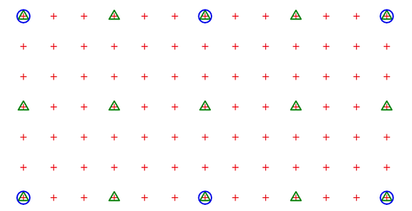
Relationship between the three grids (fine - red crosses, medium - green triangles and coarse - blue circles)
For each survey point, the fine grid is used to create facets close to the body for maximum resolution. The medium grid is used to compute a second user-defined distance. The coarse grid is used to create facets. All these facets are combined to create a general polyhedron body which is then fed to the response calculator to generate the response for that survey point.
For further information on the Terrain Correction calculator refer to the ModelVision User Guide document.
2. 3D Model Generator
This is a more user-friendly and efficient method in ModelVision for terrain correction. It intersects a polygon defining the area of interest with a terrain grid, and then triangulates the surface using compression technology to reduce the number of facets. This reduces the computation effort where surfaces are planar.
Note that this approach gives the direct terrain response rather than a correction term like is derived with traditional inner/out radii (e.g. Hammer) methods. Therefore, subtract this direct terrain response from free air gravity values, not the Bouguer corrected gravity like is done with the “typical” terrain correction approaches.
NOTE: If you are attempting to correct gravity gradiometer data, then this method is advised because it produces a faceted surface with no steps in the surface.
The 3D Model Generator can be accessed from the toolbar button or from the Model>Body Operations menu. For a step-by-step guide to using the 3D Model Generator please refer to the ModelVision User Guide or Tutorials document found in the Help>Guides menu.
3. Create Strata
The Create Strata tool is found in the toolbar button of the same name or the Model>Body Operations menu. However, as it builds a 3D faceted body directly from the grid with no compression used, the result is a computationally intense model, therefore it is not recommended before attempting the other methods available in ModelVision. Further information on this toolcan be found in the ModelVision User Guide document accessed from the Help>Guides menu.
Note: If you are only looking to PROCESS gravity data, ModelVision may not be the optimum choice of software. If however, you then want to proceed to model the data, ModelVision is the foremost software package you can use. ModelVision is used by many leading mineral exploration companies as their primary software for modelling gravity and magnetic data.
How is the Koenigsberger (Q) ratio and NRM-intensity calculated in ModelVision?
The Koenigsberger ratio Q is the ratio of the remanent magnetization to the induced magnetization. Using the abbreviations in the Body Properties dialog the formula is:
NRM Intensity/Jind
The susceptibility is in SI units but in version 12.0 and earlier, the magnetization units are in gamma rather than A/m (as expected for SI). This was changed to SI in version 13.0. This can be tested by changing the calculation mode to CGS units in the File>Project Properties dialog.
How do I import and display ModelVison .TKM files in Discover PA?
There are two options:
a) TKM files can be handled as 3D .EGB images. They can therefore be displayed either by opening from within an Image
branch, or by dragging and dropping directly into the Discover 3D window.
b) Alternatively, import your .TKM file into a Feature Database (Features>Import). This will also allow the import of any attributes
if imported into a new feature database, using the TKM file's fields as a template.
QuickDepth
The following errors may occur when processing the line data in the Data Loading dialog of QuickDepth. This could indicate that the program has detected nulls present in the dataset or the data has not been processed correctly. ModelVision will proceed to display a series of these error messages for each line in the dataset while it analyses the data.

-
Use the Delete option to delete this line from the currently saved session.
-
Use the Skip option to ignore this line in the data processing.
-
Use the Abort option to stop the progression of the data processing if you would like to analyse your input data using Utility>Statistics or visually analyse your data in map view. You can then attempt to process the grid and line data again.
When processing input data using the Data Loading dialog of QuickDepth the following message appears:
“Unable to find or create NSSFUC channel”
-
First check that the IGRF is set to the correct value for the survey data.
-
If this does not improve the data processing, then the error message could be an indicator that there are invalid/null values in the grid or line data. ModelVision cannot handle huge projects for QuickDepth because the grids are retained in memory during processing. Therefore, to manage real survey data, the Clip Project tool can be used to clip the grid and lines to a bounding rectangle, to reduce the size of the dataset and grid that is handled by QuickDepth. This means that on occasions, a start or end point on a line could have no grid value beneath it. For most operations in ModelVision this is not a problem until you must resample the grid onto the line, which is the operation in QuickDepth.
-
In the case where nulls are present at the end of lines, using the Trim Trailing Nulls tool in the Utility>Data Maintenance>Line menu to remove these.
-
In the case where non-coincident entire lines are present use the Utility>Data Maintenance>Line to Delete the offending line(s).
-
What is the gravity modelling technique in ModelVision when using the background density?
In ModelVision, the amplitude of the gravity or magnetic anomaly of a body is proportional to the difference between its property (density or magnetic susceptibility) and the background (density or magnetic susceptibility). If a body has the same property as background, then it will generate no anomaly.
With magnetic modelling we almost always set the background susceptibility to 0 and consider the absolute susceptibility values of targets. With gravity you can generally choose a background density value.
If you want to model free air data and include terrain in the model, the background density must be 0, with true densities for the rocks. If you are modelling Bouguer data then you can choose your background density. If for instance you are modelling variation in thickness of overburden on bedrock, by setting the background density to represent the bedrock, you only need a body for the overburden.
In a case of three distinct densities (representing kimberlite, limestone and granite), if your granite/limestone interface is very extensive and flat then it will generate no change in gravity. Therefore, you can make one body for the kimberlite intruding limestone, and a second body beneath it for the kimberlite intruding granite. If you set the background density to 0 then the first body would have a density of (kimberlite – limestone) and the deeper body would have a density of (kimberlite – granite). You will not need bodies for the granite or the limestone.
Assume (values are nominal only) limestone = 2.9 gm/cc, granite = 2.65, kimberlite = 2.4. Then set background density to zero and have one body of “kimberlite in limestone” with density = 2.4-2.9 = -0.5 gm/cc, and beneath it “kimberlite in granite” with density = 2.4-2.65 = -0.25 gm/cc.
However, where the geometry is more complicated and you must include gravity variations caused by the geometry of the limestone/granite interface, you may need to overlap bodies. In this case, each volume of a body overlap has an effective density contrast given by the sum of the contrast of each of the overlapping bodies against background. In the case of having overlapping bodies it is most convenient (but not necessary) to have the background density = 0.
For example, referencing the above densities, follow the steps below:
-
set background density = 0 and let this represent the granite (true density 2.65). You do not need any granite body.
-
A block of limestone by itself has a density of (2.9-2.65 = 0.25 gm/cc).
-
The kimberlite intruding the granite has a density of (2.4-2.65 = -0.25 gm/cc).
-
The kimberlite intruding the limestone also needs a contrast of -0.25 gm/cc, but if you are using a body for the limestone then the volume occupied by the kimberlite intruded into it already has a contrast of +0.25 gm/cc. You therefore need to give the “kimberlite in limestone” body a density of -0.5 gm/cc to take that contrast from +0.25 to -0.25.
Obviously, try to avoid the need to overlap bodies, although this is not always possible.
Normalised Source Strength Grid Filter
The Normalised Signal Strength (NSS) grid filter does not produce a sensible output grid.
A few suggestions to improve the result include:
-
If there are spaces in the grid name, try renaming it to one word (e.g. change “Pseudo Layer” to “TMI”) using the Utility>Data maintenance>Grid>Rename option and then re-run the NSS filter.
-
Check the dimensions of your source grid with regards, to rows x columns. The grid file may be too big. As a guide use a grid size of 1000 x 1000 for the 2D filters in ModelVision.
-
Create a subset of the ModelVision project by cropping it down to approximately 25% of the area (use the Clip Project toolbar button). Then re-run the NSS filter.
Target Wizard Tool
The cross-section views after using the Target Wizard tool do not show any data.
-
Check in the Line Control dialog (found in the Model>Line Control menu) that the Model Magnetics option is active and an Input Channel is nominated.
-
Confirm that the line data has correct/sensible easting and northing and input magnetic values.
-
When drawing the target boundary ensure that the selected target area of the anomaly is large enough to include more of the background information. This will ensure that the target wizard can pick up the highs and lows of the anomaly.
Remanence in ModelVision
How to model data when remanence is present in the data
Magnetisations that give rise to measured magnetic field anomalies are the vector sum of induced and remanent magnetisations. This magnetisation is called the Resultant Magnetisation Vector. An induced magnetisation has the same direction as the ambient earth’s geomagnetic field (except in extreme cases of anisotropy or self-demagnetisation effects) but a remanent magnetisation may be in any direction, according to its age and subsequent rotations of the rock carrying it.
Historically, remanent magnetisation has been ignored in magnetic field interpretation, but only because the relevant information about the remanent magnetisation is unavailable. The failure to correctly incorporate remanent magnetisation effects in a model can give rise to errors in the resulting estimates of the source body parameters (including size, shape, dip and position). Research shows that the resultant magnetisation is stable as an inversion parameter and is a property of the geological unit. By contrast, direct inversion for the remanent magnetisation vector can produce wildly different directions depending upon the setting of the Konigsberger ratio (Q) or magnetic susceptibility.
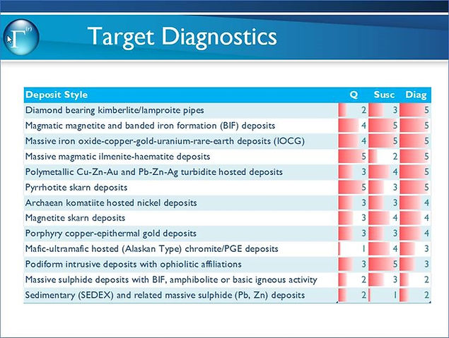
Remanence detection has high value in exploration because it indicates a geological event and is a separate property from magnetic susceptibility. The below summary was compiled by Tensor Research as part of an exhaustive review of literature on different mineralisation styles and their association with magnetic remanence.
The big breakthroughs in remanence over the last decade have been the ability to detect low levels of remanence from an isolated magnetic anomaly and the resultant magnetisation direction. The latter does not tell you the remanence direction, but it does give you some idea based on the total departure angle. This is called apparent resultant rotation angle (ARRA).
ModelVision has two methods for recovering the ARRA value. One is the Remanence Calculator tool (REMCAL) and the other is direct inversion for the remanent magnetisation vector or the resultant magnetisation vector.

Illustration of the relationship between the induced, remanent and resultant magnetisation vectors
After creating a body in ModelVision it is necessary to enable the calculation of this vector from the Body Properties dialog.

Enable the remanence computations by selecting the NRM screen in the Body Properties dialog for a generated body and enter the remanence properties. To gain access to the remanence properties first click on the Remanence check box at the bottom of the NRM screen.
For further reading on the computation of remanence in ModelVision please read “The remote determination of magnetic remanence” Pratt, et al, 2012ASEGVersion: